import matplotlib
from mpdaf.obj import mag2flux, flux2mag
from matplotlib import pyplot as plt
import numpy as np
from astropy.table import Table
matplotlib.rcParams.update({'font.size': 20})
import warnings
warnings.filterwarnings("ignore")

from pyetc.wst import WST
from pyetc.etc import show_noise, get_seeing_fwhm

Initialise ETC module

We start by creating the wst object with wst = WST(). To get more or less message, it is possible to use wst = WST(log='DEBUG') or wst = WST(log='WARNING') to have less.

wst = WST(log='INFO')

The implemented instruments are the IFS (2 channels blue and red), the MOS-LR (3 channels blue, orange and red) and the MOS-HR (4 channels U,B,V,I)

• The IFS channels are based on 4K CCD with a f/1 camera, leading to 0.25 arcsec spaxel. The LSF of 2.5 pixels, throughputs are inspired by MUSE and BlueMUSE. Note that the throughputs curves are for the telescope + instrument (excluding atmosphere).

• The MOS-LR channels are based on 6k detectors. Throughputs are inspired by 4MOST. Fiber have a 1 arcsec sky aperture. Sampling is 0.25 arcsec.

• The MOS-HR channels are based on a 9k detector. Fiber have a 0.94 arcsec sky aperture.

• In addition, paranal sky absorption and emssion are pre-computed for different conditions:

  • Moon : darksky (new moon), greysky (FLI = 0.5) and brightsky (full moon)

  • Airmass: 1, 1.2, 1.5, 2.0

  • Sky are computed with the ESO skycalc tool, using the proper spectral binning and LSF convolution for each channel

the detail of the configuration is shown with wst.info()

wst.info()

[INFO] WST ETC version: 0.3
[INFO] Telescope Cass design version Busyweek Oct 2023
[INFO] Diameter: 12.00 m Area: 100.0 m2
[INFO] IFS type IFS Channel blue
[INFO]   Inspired from BlueMUSE throughput
[INFO]   version 0.1 10/02/2023
[INFO]   Obscuration 0.180
[INFO]   Spaxel size: 0.25 arcsec Image Quality tel+ins fwhm: 0.10 arcsec beta: 2.50
[INFO]   Wavelength range [3700. 6100.] A step 0.64 A LSF 2.5 pix Npix 3751
[INFO]   Instrument transmission peak 0.38 at 5315 - min 0.28 at 3700
[INFO]   Detector RON 3.0 e- Dark 3.0 e-/h
[INFO] IFS type IFS Channel red
[INFO]   Inspired from MUSE throughput
[INFO]   version 0.1 10/02/2023
[INFO]   Obscuration 0.180
[INFO]   Spaxel size: 0.25 arcsec Image Quality tel+ins fwhm: 0.10 arcsec beta: 2.50
[INFO]   Wavelength range [6000.   9599.67] A step 0.97 A LSF 2.5 pix Npix 3712
[INFO]   Instrument transmission peak 0.39 at 6830 - min 0.08 at 9600
[INFO]   Detector RON 3.0 e- Dark 3.0 e-/h
[INFO] MOSLR type MOS Channel blue
[INFO]   Inspired from 4MOST LR throughput
[INFO]   version 0.2 30/11/2023
[INFO]   Obscuration 0.100
[INFO]   Spaxel size: 0.25 arcsec Image Quality tel+ins fwhm: 0.30 arcsec beta: 2.50
[INFO]   Fiber aperture: 1.0 arcsec
[INFO]   Wavelength range [3700.   5349.84] A step 0.41 A LSF 4.1 pix Npix 4025
[INFO]   Instrument transmission peak 0.40 at 4932 - min 0.03 at 3700
[INFO]   Detector RON 3.0 e- Dark 3.0 e-/h
[INFO] MOSLR type MOS Channel orange
[INFO]   Inspired from 4MOST LR throughput
[INFO]   version 0.2 30/11/2023
[INFO]   Obscuration 0.100
[INFO]   Spaxel size: 0.25 arcsec Image Quality tel+ins fwhm: 0.30 arcsec beta: 2.50
[INFO]   Fiber aperture: 1.0 arcsec
[INFO]   Wavelength range [5150.  7399.5] A step 0.55 A LSF 4.1 pix Npix 4091
[INFO]   Instrument transmission peak 0.41 at 6435 - min 0.16 at 5150
[INFO]   Detector RON 3.0 e- Dark 3.0 e-/h
[INFO] MOSLR type MOS Channel red
[INFO]   Inspired from 4MOST LR throughput
[INFO]   version 0.2 30/11/2023
[INFO]   Obscuration 0.100
[INFO]   Spaxel size: 0.25 arcsec Image Quality tel+ins fwhm: 0.30 arcsec beta: 2.50
[INFO]   Fiber aperture: 1.0 arcsec
[INFO]   Wavelength range [7200.   9699.78] A step 0.61 A LSF 4.1 pix Npix 4099
[INFO]   Instrument transmission peak 0.38 at 7983 - min 0.09 at 9700
[INFO]   Detector RON 3.0 e- Dark 3.0 e-/h
[INFO] MOSHR type MOS Channel U
[INFO]   WST HR spectrometer possible baseline description
[INFO]   version 1.1 13/02/2023
[INFO]   Obscuration 0.000
[INFO]   Spaxel size: 0.22 arcsec Image Quality tel+ins fwhm: 0.30 arcsec beta: 2.50
[INFO]   Fiber aperture: 0.9 arcsec
[INFO]   Wavelength range [3800.     3999.9872] A step 0.02 A LSF 4.5 pix Npix 9217
[INFO]   Instrument transmission peak 0.12 at 3994 - min 0.07 at 3800
[INFO]   Detector RON 3.0 e- Dark 3.0 e-/h
[INFO] MOSHR type MOS Channel B
[INFO]   WST HR spectrometer possible baseline description
[INFO]   version 1.1 13/02/2023
[INFO]   Obscuration 0.000
[INFO]   Spaxel size: 0.21 arcsec Image Quality tel+ins fwhm: 0.30 arcsec beta: 2.50
[INFO]   Fiber aperture: 0.9 arcsec
[INFO]   Wavelength range [5067.    5331.973] A step 0.03 A LSF 4.5 pix Npix 9138
[INFO]   Instrument transmission peak 0.13 at 5237 - min 0.11 at 5067
[INFO]   Detector RON 3.0 e- Dark 3.0 e-/h
[INFO] MOSHR type MOS Channel V
[INFO]   WST HR spectrometer possible baseline description
[INFO]   version 1.1 13/02/2023
[INFO]   Obscuration 0.000
[INFO]   Spaxel size: 0.21 arcsec Image Quality tel+ins fwhm: 0.30 arcsec beta: 2.50
[INFO]   Fiber aperture: 0.9 arcsec
[INFO]   Wavelength range [6431.     6767.9794] A step 0.04 A LSF 4.5 pix Npix 9183
[INFO]   Instrument transmission peak 0.13 at 6654 - min 0.11 at 6431
[INFO]   Detector RON 3.0 e- Dark 3.0 e-/h
[INFO] MOSHR type MOS Channel I
[INFO]   WST HR spectrometer possible baseline description
[INFO]   version 1.1 13/02/2023
[INFO]   Obscuration 0.000
[INFO]   Spaxel size: 0.21 arcsec Image Quality tel+ins fwhm: 0.30 arcsec beta: 2.50
[INFO]   Fiber aperture: 0.9 arcsec
[INFO]   Wavelength range [8380.    8819.999] A step 0.05 A LSF 4.5 pix Npix 9206
[INFO]   Instrument transmission peak 0.13 at 8657 - min 0.10 at 8381
[INFO]   Detector RON 3.0 e- Dark 3.0 e-/h

Instruments and channels

The wst object has one telescope and two instruments: wst.tel, wst.ifs and wst.moslr. Each instrument has 2 channels: blue and red. For example, to access the red channel of the ifs we have to use wst.ifs['red']. Each channel is a dictionary with all instrument properties.

For example to list all elements of the MOS-LR blue channel, we will use wst.moslr['blue'].keys().

wst.moslr['blue'].keys()

dict_keys(['desc', 'version', 'ref', 'type', 'obscuration', 'iq_fwhm', 'iq_beta', 'spaxel_size', 'aperture', 'dlbda', 'lbda1', 'lbda2', 'lsfpix', 'ron', 'dcurrent', 'wave', 'sky', 'instrans', 'skys', 'chan', 'name'])

The dictionary keys are the following:

• desc: description of the channel

• version: version of the channel

• ref: reference for this version

• name: channel name (eg ifs or moslr)

• chan: channel name (blue or red)

• type: instrument type (IFS or MOS)

• obscuration: fraction of light loss in the telescope path (could be different from MOS and IFS)

• iq_fwhm: the FWHM of the image quality of telescope + instrument, excluding atmosphere

• iq_beta: the beta parameter of the MOFFAT image quality

• aperture: the fiber diameter aperture in arcsec (only for MOS)

• spaxel_size: the spaxel size in arcsec

• dlbda: the wavelength increment in A

• lbda1: starting wavelength in A

• lbda2: ending wavelength in A

• lsfpix: the LSF size in spectels (spectral pixels)

• ron: read-out noise in e- by pixel

• dcurrent: dark current in e-/hour by pixel

• wave: wavelength WaveCoord MPDAF object (see MPDAF spectrum documentation)

• instrans: total telescope + instrument transmission, excluding atmosphere (Spectrum MPDAF object)

• skys: the list of the name of all moon configuration e.g. wst.ifs['blue']['skys'] = ['brightsky', 'darksky', 'greysky']

• sky: a list of dictionnaries related to each sky configuration

One can view them the first one with wst.ifs['blue']['sky'][0]

wst.ifs['blue']['sky'][0]

{'moon': 'brightsky',
 'airmass': 1.0,
 'emi': <Spectrum(shape=(3751,), unit='', dtype='>f8')>,
 'abs': <Spectrum(shape=(3751,), unit='', dtype='>f8')>,
 'filename': '/Users/rolandbacon/Library/CloudStorage/Dropbox/Soft/python/pyetc/pyetc/data/WST/ifs_blue_brightsky_1.0.fits'}

Spectral resolution

We now note ins a specific instrument channel, eg ins = wst.ifs['red'] The function ins.get_spectral_resolution() return an array with the spectral resolution. The ins['wave'].coord()return the corresponding wavelength array.

fig,ax = plt.subplots(1,3,figsize=(18,5))
ax[0].plot(wst.ifs['blue']['wave'].coord(), wst.get_spectral_resolution(wst.ifs['blue']), color='b')
ax[0].plot(wst.ifs['red']['wave'].coord(), wst.get_spectral_resolution(wst.ifs['red']), color='r')
ax[1].plot(wst.moslr['blue']['wave'].coord(), wst.get_spectral_resolution(wst.moslr['blue']), color='b')
ax[1].plot(wst.moslr['orange']['wave'].coord(), wst.get_spectral_resolution(wst.moslr['orange']), color='orange')
ax[1].plot(wst.moslr['red']['wave'].coord(), wst.get_spectral_resolution(wst.moslr['red']), color='r')
ax[2].plot(wst.moshr['U']['wave'].coord(), wst.get_spectral_resolution(wst.moshr['U']), color='m')
ax[2].plot(wst.moshr['B']['wave'].coord(), wst.get_spectral_resolution(wst.moshr['B']), color='b')
ax[2].plot(wst.moshr['V']['wave'].coord(), wst.get_spectral_resolution(wst.moshr['V']), color='g')
ax[2].plot(wst.moshr['I']['wave'].coord(), wst.get_spectral_resolution(wst.moshr['I']), color='r')


ax[0].set_xlabel('Wavelength (A)')
ax[1].set_xlabel('Wavelength (A)')
ax[2].set_xlabel('Wavelength (A)')
ax[0].set_ylabel('Spectral resolution')
ax[0].set_title('IFS')
ax[1].set_title('MOS-LR');
ax[2].set_title('MOS-HR');

Throughput

The ins['instrans'] is a MPDAF spectrum with the total instrument plus telescope throughput.

fig,ax = plt.subplots(1,3,figsize=(18,5), sharey=True)
ax[0].plot(wst.ifs['blue']['instrans'].wave.coord(), wst.ifs['blue']['instrans'].data)
ax[0].plot(wst.ifs['red']['instrans'].wave.coord(), wst.ifs['red']['instrans'].data)
ax[1].plot(wst.moslr['blue']['instrans'].wave.coord(), wst.moslr['blue']['instrans'].data)
ax[1].plot(wst.moslr['orange']['instrans'].wave.coord(),wst.moslr['orange']['instrans'].data)
ax[1].plot(wst.moslr['red']['instrans'].wave.coord(),wst.moslr['red']['instrans'].data)
for chan in wst.moshr['channels']:
    ax[2].plot(wst.moshr[chan]['instrans'].wave.coord(),wst.moshr[chan]['instrans'].data)
ax[0].set_xlabel(r'Wavelength ($\AA$)')
ax[1].set_xlabel(r'Wavelength ($\AA$)')
ax[2].set_xlabel(r'Wavelength ($\AA$)')
ax[0].set_ylabel('Total Throughput (excl atm)')
ax[0].set_title('IFS')
ax[1].set_title('MOS-LR');
ax[2].set_title('MOS-HR');

Surface Brightness

We now derive S/N estimate for surface brightness sources. In this case the source is just defined by a spectrum. The function spec = wst.get_spec(ins, dspec) is used to build the source spectrum. The dspec dictionnary has the spectrum parameters, there are currently three categories of sources: flatcont, line and template.

The flatcont type describe a flat continuum source: dict(type='flatcont', wave=[lbda1,lbda2]) where wave is the wavelength range, in A. The result of the get_spec function is a MPDAF spectrum. The spectrum is normalized at 1. See here for the MPDAF Spectrum documentation.

ifs = wst.ifs['red']
wave = 8000
dspec = dict(type='flatcont', wave=[wave-10,wave+10])
spec = wst.get_spec(ifs, dspec)
spec.plot()

The line type, describe an emission line. The emission line is modelled by a skewed gaussin function with the following parameters: dict(type='line', lbda=wave, sigma=4.0, skew=7.0) where wave is the wavelength of the peak, sigma is the gaussian sigma and skew is the skew parameter. A Gaussian has skew=0.

wave = 8000
dspec = dict(type='line', lbda=wave, sigma=4.0, skew=7.0)
spec = wst.get_spec(ifs, dspec)
spec.plot()

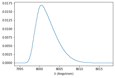
By default, the returned emission line spectrum is oversampled by a factor 10 with respect to the instrument spctral sampling and convolved with the LSF. The rebinning and trunctation of the spectral is performed later. It is possible to change this parameters, but it is recommneded to keep the default LSF convolution and oversampling.

spec = wst.get_spec(ifs, dspec, oversamp=1, lsfconv=False)
spec.plot()

The template type describe one of the source of the spextra python library. Check the documentation here for the complete list. The parameters are the following: - name, the name of the template - redshift, the redshift to apply to the template (if not set, the template is not redshifted) - wave_center, the central wavelength in A used to normalize the spectrum - wave_wdth, the window in A used for the normailsation

Note that window does not need to be within the channel wavelngth interval. The template spectrum is LSF convolved and resampled to the channel sampling.

ifs = wst.ifs['red']
wave,dw = 6000,500
dspec = dict(type='template', name='kc96/starb1', redshift=0.5,
             wave_center=wave, wave_width=dw)
spec = wst.get_spec(ifs, dspec)
spec.plot()

The next step is to define the observation parameters. They are written in a dictionnary which is add to the wst object by the wst.set_obs(obs) command.

The content of wst.obs is function of the source type. For surface brightness source it is composed of:

• moon: the moon phase, it must be part of the pre-loaded configurations (currently darksky, greysky or brightsky).

• airmass: the observation airmass. Note that it must be part of the pre-loaded sky configuration, otherwise the program will raise an exception.

• ndit: the number of exposures

• dit: the integration time of one exposure in sec

• ima_type: sb, for surface brightness

• ima_area: the size of the area to be considered for S/N computation. It is needed only for IFS, for the MOS it is defined by the fiber aperture.

• spec_type: must be one of cont,line,template

in addition if spec_type is set to line, additional parameters are needed: - spec_range_type: can be fixed or adaptative, used to define the spectral range to consider for the S/N computation. - spec_range_hsize_spectels: if spec_range_type is fixed, it define the number of spectels to consider, the total size is 2 * spec_range_hsize_spectels + 1 - spec_range_kfwhm: if spec_range_type is adaptative, it compute the size of the window relative to the FWHM of the line.

The last parameter needed is the flux of the source in \(erg.s^{-1}.cm^{-2}.arcsec^{-2}\) unit.

Continuum source

obs = dict(
    moon='darksky',
    airmass = 1.0,
    ndit = 2,
    dit = 1800,
    spec_type = 'cont',
    ima_type = 'sb',
    ima_area = 1.0
)
wst.set_obs(obs)

The estimate of S/N is then computed with the wst.snr_from_source() command.

Note that the ima parameter is set to None because we are in the surface brightness mode.

flux = 5.e-19
res = wst.snr_from_source(ifs, flux, ima=None, spec=spec)

The output of snr_from_source is the dictionary res. It contains the following elements:

• input: a dictionnary with some input data used in S/N computation

• cube: a dictionary that contains S/N measurements by voxels

• spec: a dictionnary that contains S/N summed over the spatial direction

• aper: a dictionnary with values summed over an aperture (only for line spectral type)

We detail the content of each dictionnary in the next paragraphs.

The input dictionary contains the following items:

• flux_source: the source flux in erg/s/cm2/voxel

• atm_abs: the atmospheric absorption

• atm_emi: the atmospheric emission in e-/s

• and all used obs parameters

res['input']

{'flux_source': <Spectrum(shape=(3712,), unit='', dtype='float64')>,
 'atm_abs': <Spectrum(shape=(3712,), unit='', dtype='>f8')>,
 'ins_trans': <Spectrum(shape=(3712,), unit='', dtype='float64')>,
 'atm_emi': <Spectrum(shape=(3712,), unit='', dtype='>f8')>,
 'dl': 0.97,
 'flux': 5e-19,
 'moon': 'darksky',
 'dit': 1800,
 'ndit': 2,
 'airmass': 1.0,
 'spec_type': 'cont',
 'ima_type': 'sb',
 'ima_area': 1.0}

r = res['input']
fig,ax = plt.subplots(1,3,figsize=(18,5))
r['flux_source'].plot(ax=ax[0], title='flux_source')
r['atm_abs'].plot(ax=ax[1], title='atm_abs')
r['atm_emi'].plot(ax=ax[2], title='atm_emi')

The cube dictionary contains all quantities by voxels. Depending of the type of the source it can be datacubes, images or spectra. In the case of surface brightness source, it is restricted to spectra, because all spaxels are identical.

• snr: the snr spectrum by voxel which can be displayed with snr.plot().

• noise: the noise dictionnary contains all sources of noise by voxel.

  • ron: the detector readout noise in e- (constant with wavelength)

  • dark: the detector dark current in e- (cosntant with wavelength)

  • sky: the sky noise spectrum in e-

  • source: the source noise spectrum in e-

  • tot: the total noise spectrum in e-

• nph_source: the number of source photo-electrons received by voxel

• nph_sky: the number of source photo-electrons received by voxel

The show_noise(res['cube']['noise'], ax) can be used to display the relative noise contrbution.

One can see in this example, that we are in photon noise regime, with 80% of the noise contribution due to the sky brightness.

fig,ax = plt.subplots(2,1,figsize=(12,12))
res['cube']['snr'].plot(ax=ax[1])
ax[0].set_ylabel('S/N by voxel')
show_noise(res['cube']['noise'], ax[0], legend=True)
ax[1].set_ylabel('Relative noise contribution by voxel');

fig,ax = plt.subplots(1,2,figsize=(18,5))
res['cube']['nph_source'].plot(ax=ax[0], stretch='log', title='source e-/voxel')
res['cube']['nph_sky'].plot(ax=ax[1], stretch='log', title='sky e-/voxel')

The spec dictionary contains all spatially integrated quantities, in MPDAF spectrum format. Specifically it is composed of:

• frac_flux: the total fraction of flux recovered (it is 1 in our case)

• frac_ima: thre fraction of flux recoovered in the spatial axis

• frac_spec: thre fraction of flux recoovered in the spectral axis

• nb_spaxels: the number of spaxels that have been summed

• nph_source: the number of source photo-electrons received by spectel

• nph_sky: the number of source photo-electrons received by spectel

• snr: the snr spectrum by spectel

• snr_mean: the average value of the S/N by spectels

• snr_min: the minimum value of the S/N by spectels

• snr_max: the maximum value of the S/N by spectels

• noise: the noise dictionnary contains all sources of noise by spectel.

  • ron: the detector readout noise in e- (constant with wavelength)

  • dark: the detector dark current in e- (cosntant with wavelength)

  • sky: the sky noise spectrum in e-

  • source: the source noise spectrum in e-

  • tot: the total noise spectrum in e-

fig,ax = plt.subplots(1,1,figsize=(12,5))
sp = res['spec']
sp['snr'].plot(ax=ax, title=r'S/N achieved in the 1 $arcsec^2$ area')
ax.text(0.9, 0.9, f"S/N mean {sp['snr_mean']:.2f} min {sp['snr_min']:.2f} max {sp['snr_max']:.2f}",
       transform=ax.transAxes, ha='right', va='top')

Text(0.9, 0.9, 'S/N mean 2.64 min 0.19 max 22.84')

Emission line source

Computation for an emission line extended source is similar. This gives:

wave = 8000
dspec = dict(type='line', lbda=wave, sigma=4.0, skew=7.0)
spec = wst.get_spec(ifs, dspec)
obs = dict(
    moon='darksky',
    airmass = 1.2,
    ndit = 2,
    dit = 1800,
    spec_type = 'line',
    spec_range_type = 'fixed',
    spec_range_hsize_spectels = 7,
    ima_type = 'sb',
    ima_area = 1.0,
)
wst.set_obs(obs)
flux = 1.e-18
res = wst.snr_from_source(ifs, flux, ima=None, spec=spec)

The res dictionary now contains an additional item: aper. This new directory contains measurements once integrated both spatially and spectrally. Specifically it contains:

• frac_flux: the total fraction of captured flux

• frac_ima: the fraction of flux captured within the spatial aperture

• frac_spec: the fraction of flux captured along the spectral direction

• nb_spaxels: the number of summed spaxels

• nb_spectels: the number of summed spectels

• nb_voxels: the total number of summed voxels

• nph_source: the number of source photo-electrons

• nph_sky: the number of sky photo-electrons

• snr: the snr spectrum

• ron: the detector readout noise in e-

• dark: the detector dark current in e-

• sky_noise: the sky noise in e-

• source_noise: the source noise in e-

• tot_noise: the total noise in e-

• frac_detnoise: the ratio of the detector (ron+dark) variance to the total variance

The wst.print_aper(res, title) can be used to display the result

wst.print_aper(res, 'aperture values')

Table length=17

item	aperture values
bytes20	bytes20
snr	0.7733
size	1
area	1
frac_flux	0.962
frac_ima	1
frac_spec	0.962
nb_spaxels	16
nb_spectels	15
nb_voxels	240
nph_source	316.4
nph_sky	1.624e+05
ron	65.73
dark	26.83
sky_noise	403
source_noise	17.79
tot_noise	409.2
frac_detnoise	0.0301

The cube dictionary contains an additional element: trunc_spec which the spectrum after truncation by a window specified by the spec_range_hsize_spectels obs keyword. It is displayed here:

fig,ax = plt.subplots(1,2,figsize=(18,5))
spec.plot(ax=ax[0], title='original oversampled spec')
res['cube']['trunc_spec'].plot(ax=ax[1], title=f"trunc_spec [fixed window S/N {res['aper']['snr']:.2f}]")

Rather than using a window of fixed size, we can use an adaptative size which is function of the fwhm of the line.

obs = dict(
    moon='darksky',
    airmass = 1.2,
    ndit = 2,
    dit = 1800,
    spec_type = 'line',
    spec_range_type = 'adaptative',
    spec_range_kfwhm = 2,
    ima_type = 'sb',
    ima_area = 1.0,
)
wst.set_obs(obs)
res = wst.snr_from_source(ifs, flux, ima=None, spec=spec)

fig,ax = plt.subplots(1,2,figsize=(18,5))
spec.plot(ax=ax[0], title='original oversampled spec')
res['cube']['trunc_spec'].plot(ax=ax[1], title=f"trunc_spec [adaptative window S/N {res['aper']['snr']:.2f}]")

We see that the adptative window better follow the asymetric line shape and provide a S/N improved by a factor 2.

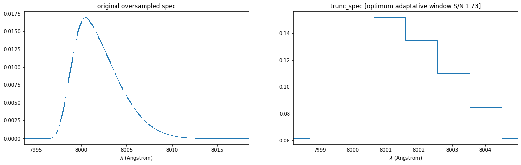
We can go one step further by using the wst.optimum_spectral_range() function to find the spec_range_fkwhm parameter whihc maximize the S/N. The optimum parameter is saved in the obs parameters, so we just need to rerun snr_from_source after.

kfwhm = wst.optimum_spectral_range(ifs, flux, None, spec)
res = wst.snr_from_source(ifs, flux, ima=None, spec=spec)

fig,ax = plt.subplots(1,2,figsize=(18,5))
spec.plot(ax=ax[0], title='original oversampled spec')
res['cube']['trunc_spec'].plot(ax=ax[1], title=f"trunc_spec [optimum adaptative window S/N {res['aper']['snr']:.2f}]")

Retrieve flux for a given S/N

It is often useful to evaluate the flux limit, i.e. the flux which is needed to obtain a S/N of 3. For this, we can use the wst.flux_from_source function.

snr = 3
res = wst.flux_from_source(ifs, snr, None, spec)

In the case of an emission line source, the estimated flux value is saved in res['aper']['flux'].

wst.print_aper(res, 'res')

Table length=18

item	res
bytes20	bytes20
snr	3
size	1
area	1
frac_flux	0.8643
frac_ima	1
frac_spec	0.8643
nb_spaxels	16
nb_spectels	8
nb_voxels	128
nph_source	496
nph_sky	2.415e+04
ron	48
dark	19.6
sky_noise	155.4
source_noise	22.27
tot_noise	165.3
frac_detnoise	0.09835
flux	1.745e-18

But in the case of a cont or template source, we have to specify a window range to compute an average target S/N. This is done with the snrcomp dictionary which specify a method and a wavelength range (waves) of the wst.flux_from_source function. Here is an example:

wave,dw = 6000,500
dspec = dict(type='template', name='kc96/starb1',
             wave_center=wave, wave_width=dw)
spec = wst.get_spec(ifs, dspec)
obs = dict(
    moon = 'darksky',
    airmass = 1.0,
    ndit = 2,
    dit = 1800,
    spec_type = 'cont',
    ima_type = 'sb',
    ima_area = 1.0
)
wst.set_obs(obs)
snr = 3
res = wst.flux_from_source(ifs, snr, None, spec, snrcomp=dict(method='mean', waves=[7000,8000]))

fig,ax = plt.subplots(1,1,figsize=(12,5))
res['spec']['snr'].plot(ax=ax)
ax.set_title(f"S/N for flux {res['spec']['flux']:.2e} "+r"$erg.s^{-1}.cm^{-2}.arcsec^{-2}$ (area $1 arcsec^2$)")
ax.axhline(3, color='r');

Point Source

All objects with a size much smaller than the PSF are considered as point source. Their shape is given by the predicted atmospheric + telescope + instrument PSF. The atmospheric seeing limited model is taken from the ESO VLT ETC, adapted to the larger size of the WST. The telescope plus instrument image quality is currently estimated to be 0.1 arcsec FWHM for the IFS and 0.3 arcsec FWHM for the MOS.

Image Quality

Here is the total PSF at zenith for a seeing of 0.7 arcsec @ 500 nm.

fig,ax = plt.subplots(1,1,figsize=(12,5))
seeing = 0.7
airmass = 1
for ins in [wst.ifs, wst.moslr]:
    for chan in ins['channels']:
        inst = ins[chan]
        wave = inst['wave'].coord()
        fwhm = get_seeing_fwhm(seeing, airmass, wave, wst.tel['diameter'], inst['iq_fwhm'])
        ax.plot(wave, fwhm, label=f"{inst['name']} {chan}")
ax.legend()

<matplotlib.legend.Legend at 0x7f8e713e63a0>

Continuum source

To compute the S/N for a point source, we need to define the spectrum and the seeing and airmass of the observation. The ima_type is set to ps. Here is an example for a sun-like star with V AB mag of 23.

mos = wst.moslr['blue']
wave,dw  = 5500,500
dspec = dict(type='template', name='ref/sun',
             wave_center=wave, wave_width=dw)
spec = wst.get_spec(mos, dspec)
mag = 23
flux = mag2flux(mag, wave)
obs = dict(
    moon = 'brightsky',
    seeing = 0.7,
    airmass = 1.0,
    ndit = 2,
    dit = 1800,
    spec_type = 'cont',
    ima_type = 'ps',
)
wst.set_obs(obs)

res = wst.snr_from_source(mos, flux, None, spec)

fig,ax = plt.subplots(1,3,figsize=(18,5))
res['input']['flux_source'].plot(ax=ax[0], title='Input Flux')
res['spec']['snr'].plot(ax=ax[1], title='S/N')
show_noise(res['spec']['noise'], ax=ax[2])

One can see that we are readout noise limited below 4000 A.

To perform the same computation with the IFS we need to define further parameters for the aperture. While it is fixed by the fiber aperture in the MOS design, for the IFS we have the choice between circular_adaptative or square_fixed. As indicated by its name square_fixed use a square aperture with a fixed size in spaxels defined by 2 x ima_aperture_hsize_spaxels + 1 spaxels.

The circular_adaptative method, is relative to the FWHM size of the image and use the ima_kfwhm parameter. As for the spectrum, it can be optimized using the optimum_circular_aperture method.

We show an example using the same source with the IFS blue channel. Note that for the optimsation we have to define thelrangeparameter in the routine

ifs = wst.ifs['blue']
wave,dw  = 5500,500
dspec = dict(type='template', name='ref/sun',
             wave_center=wave, wave_width=dw)
spec = wst.get_spec(ifs, dspec)
mag = 23
flux = mag2flux(mag, wave)

obs = dict(
    moon = 'brightsky',
    seeing = 0.7,
    airmass = 1.0,
    ndit = 2,
    dit = 1800,
    spec_type = 'cont',
    ima_type = 'ps',
    ima_aperture_type = 'circular_adaptative',
)
wst.set_obs(obs)
kfwhm = wst.optimum_circular_aperture(ifs, flux, None, spec, lrange=[4500,5500])
res = wst.snr_from_source(ifs, flux, None, spec)

fig,ax = plt.subplots(1,3,figsize=(18,5))
res['input']['flux_source'].plot(ax=ax[0], title='Input Flux')
res['spec']['snr'].plot(ax=ax[1], title='S/N')
show_noise(res['spec']['noise'], ax=ax[2])

Emission line source

We can repeat this computation with an emission line source. The process is similar to the surface brightness computation.

mos = wst.moslr['blue']
ifs = wst.ifs['blue']
wave = 4900
dspec = dict(type='line', lbda=wave, sigma=4.0, skew=7.0)
flux= 5.e-18
obs = dict(
    moon = 'darksky',
    seeing = 0.7,
    airmass = 1.0,
    ndit = 2,
    dit = 1800,
    spec_type = 'line',
    spec_range_type = 'adaptative',
    spec_range_kfwhm = 2,
    ima_type = 'ps',
    ima_aperture_type = 'circular_adaptative',
    ima_kfwhm = 2
)
wst.set_obs(obs)
spec = wst.get_spec(ifs, dspec)
kfwhm_ima = wst.optimum_circular_aperture(ifs, flux, None, spec)
kfwhm_spec = wst.optimum_spectral_range(ifs, flux, None, spec)
res1 = wst.snr_from_source(ifs, flux, None, spec)
spec = wst.get_spec(mos, dspec)
res2 = wst.snr_from_source(mos, flux, None, spec)

The function wst.print_aper() can be used to display the tabulated differences between the MOS and the IFS

wst.print_aper([res1,res2],['ifs','mos'])

Table length=17

item	ifs	mos
bytes20	bytes20	bytes20
snr	6.974	5.201
size	1.427	1
area	1.599	0.7854
frac_flux	0.7367	0.5172
frac_ima	0.9556	0.6406
frac_spec	0.7708	0.8074
nb_spaxels	21	19
nb_spectels	9	15
nb_voxels	189	285
nph_source	853.8	709.3
nph_sky	1.017e+04	1.191e+04
ron	58.33	71.62
dark	23.81	29.24
sky_noise	100.8	109.1
source_noise	29.22	26.63
tot_noise	122.4	136.4
frac_detnoise	0.2648	0.3218

Retrieve flux for a given S/N

It is also possible to retreive the flux to achieve a given S/N. Here is an example.

mos = wst.moslr['red']
ifs = wst.ifs['red']
moon = 'darksky'
wave = 8000
dspec = dict(type='line', lbda=wave, sigma=4.0, skew=7.0)
flux= 5.e-18
obs = dict(
    moon = 'darksky',
    seeing = 0.7,
    airmass = 1.0,
    ndit = 2,
    dit = 1800,
    spec_type = 'line',
    spec_range_type = 'adaptative',
    spec_range_kfwhm = 1.2,
    ima_type = 'ps',
    ima_aperture_type = 'circular_adaptative',
    ima_kfwhm = 5
)
wst.set_obs(obs)
snr = 3
spec = wst.get_spec(ifs, dspec)
res1 = wst.flux_from_source(ifs, snr, None, spec)
spec = wst.get_spec(mos, dspec)
res2 = wst.flux_from_source(mos, snr, None, spec)

wst.print_aper([res1,res2],['ifs','mos'])

Table length=18

item	ifs	mos
bytes20	bytes20	bytes20
snr	3	3
size	0.8269	1
area	0.537	0.7854
frac_flux	0.5783	0.627
frac_ima	0.6692	0.7606
frac_spec	0.8643	0.8243
nb_spaxels	9	17
nb_spectels	8	11
nb_voxels	72	187
nph_source	350.1	532.2
nph_sky	1.175e+04	2.701e+04
ron	36	58.02
dark	14.7	23.69
sky_noise	108.4	164.3
source_noise	18.71	23.07
tot_noise	116.7	177.4
frac_detnoise	0.1111	0.1248
flux	1.826e-18	1.804e-18

Resolved source

Resolved sources are defined by an image and a spectrum. The image is computed with the wst.get_image(ins, dima) function, with ins the instrument channel and dima a dictionary describing the image model. Currentkly there are two image models, the moffat model: It is describe by a fwhm in arcsec, a beta shape parameter, and optionnally an ellipticity ell, and the sersic model: it is described by an effective radius reff in arcsec, a sersic index n, and optionnally an ellipticity ell.

ifs = wst.ifs['red']
dima = dict(type='sersic', reff=1.0, n=2.0, ell=0.6)
ima = wst.get_ima(ifs, dima)
ima.plot(zscale=True)

<matplotlib.image.AxesImage at 0x7f8e8c32f7c0>

Continuum source

In MOS instrument, the spatial aperture is fixed by the fiber diameter in arcsec.

For IFS there are two sort of apertures:

• square_fixed, the size of the aperture in spaxels is given by 2 * ima_aperture_hsize_spaxels + 1

• circular_adaptative, the aperture diameter is computed relativelt to the FWHM of the image and is given by ima_kfwhm

Note that currently no PSF convolution is done on the image

The final aperture used for the S/N computation can be found in the res[‘cube’][‘trunc_ima’] image. An example is given below:

ifs = wst.ifs['red']
wave = 8000
dspec = dict(type='flatcont', wave=[wave-10,wave+10])
spec = wst.get_spec(ifs, dspec)
dima = dict(type='moffat', fwhm=1.0, beta=2.5)
ima = wst.get_ima(ifs, dima)
mag = 23
flux = mag2flux(mag, wave)
obs = dict(
    moon = 'greysky',
    airmass = 1.0,
    ndit = 2,
    dit = 1800,
    spec_type = 'cont',
    ima_type = 'resolved',
    ima_aperture_type = 'circular_adaptative',
    ima_kfwhm = 5,
)

wst.set_obs(obs)
res1 = wst.snr_from_source(ifs, flux, ima, spec)
obs = dict(
    moon = 'greysky',
    airmass = 1.0,
    ndit = 2,
    dit = 1800,
    spec_type = 'cont',
    ima_type = 'resolved',
    ima_aperture_type = 'square_fixed',
    ima_aperture_hsize_spaxels = 2,
)
wst.set_obs(obs)
res2 = wst.snr_from_source(ifs, flux, ima, spec)

mos = wst.moslr['red']
spec = wst.get_spec(mos, dspec)
ima = wst.get_ima(mos, dima)
obs = dict(
    moon = 'greysky',
    airmass = 1.0,
    ndit = 2,
    dit = 1800,
    spec_type = 'cont',
    ima_type = 'resolved',
)
wst.set_obs(obs)
res3 = wst.snr_from_source(mos, flux, ima, spec)

fig,ax = plt.subplots(1,3,figsize=(18,5))
res1['cube']['trunc_ima'].plot(ax=ax[0], title='IFS circular_adaptative')
res2['cube']['trunc_ima'].plot(ax=ax[1], title='IFS square_fixed')
res3['cube']['trunc_ima'].plot(ax=ax[2], title='MOS')

<matplotlib.image.AxesImage at 0x7f8e8c40ca90>

As for the spectrum adaptative spectral range, it is possible for the IFS to find the optimum ima_kfwm parameter to maximize the S/N. The function wst.optimum_circular_aperture() perform this task. We illustrate this in the following.

ifs = wst.ifs['red']
wave = 7000
dspec = dict(type='flatcont', wave=[wave-10,wave+10])
spec = wst.get_spec(ifs, dspec)
dima = dict(type='moffat', fwhm=1.0, beta=2.5)
ima = wst.get_ima(ifs, dima)
mag = 23
flux = mag2flux(mag, wave)
obs = dict(
    moon = 'greysky',
    airmass = 1.0,
    ndit = 2,
    dit = 1800,
    spec_type = 'cont',
    ima_type = 'resolved',
    ima_aperture_type = 'circular_adaptative',
    ima_kfwhm = 5,
)
wst.set_obs(obs)
kfwhm = wst.optimum_circular_aperture(ifs, flux, ima, spec, lrange=[wave-5,wave+5])
res4 = wst.snr_from_source(ifs, flux, ima, spec)

for res,name in zip([res3,res2,res1,res4],['MOS','IFS square fix','IFS circular adaptative','IFS optimum circular adaptative']):
    print(f"{name} S/N mean {res['spec']['snr_mean']:.2f} min {res['spec']['snr_min']:.2f} max {res['spec']['snr_max']:.2f}")

MOS S/N mean 1.38 min 0.50 max 1.66
IFS square fix S/N mean 2.04 min 0.73 max 2.46
IFS circular adaptative S/N mean 1.82 min 0.65 max 2.19
IFS optimum circular adaptative S/N mean 3.10 min 2.73 max 3.22

Emission line source

The emission line source follow the same scheme.

ifs = wst.ifs['blue']
wave = 4900
obs = dict(
    moon='darksky',
    airmass = 1.2,
    ndit = 2,
    dit = 1800,
    spec_type = 'line',
    spec_range_type = 'adaptative',
    spec_range_kfwhm = 2,
    ima_type = 'resolved',
    ima_aperture_type = 'circular_adaptative',
    ima_kfwhm = 5,
)
wst.set_obs(obs)
flux = 1.e-18
dspec = dict(type='line', lbda=wave, sigma=4.0, skew=7.0)
spec = wst.get_spec(ifs, dspec)
dima = dict(type='moffat', fwhm=1.0, beta=2.5)
ima = wst.get_ima(ifs, dima)
flux = 5.e-18
kfwhm = wst.optimum_circular_aperture(ifs, flux, ima, spec)
kfwhm = wst.optimum_spectral_range(ifs, flux, ima, spec)
res1 = wst.snr_from_source(ifs, flux, ima, spec)
mos = wst.moslr['blue']
spec = wst.get_spec(mos, dspec)
ima = wst.get_ima(mos, dima)
kfwhm = wst.optimum_spectral_range(mos, flux, ima, spec)
res2 = wst.snr_from_source(mos, flux, ima, spec)

wst.print_aper([res1,res2],['IFS','MOS'])

Table length=17

item	IFS	MOS
bytes20	bytes20	bytes20
snr	3.465	2.734
size	1.665	1
area	2.177	0.7854
frac_flux	0.5081	0.3103
frac_ima	0.6592	0.371
frac_spec	0.7708	0.8365
nb_spaxels	37	21
nb_spectels	9	16
nb_voxels	333	336
nph_source	571.1	412.7
nph_sky	1.959e+04	1.532e+04
ron	77.42	77.77
dark	31.61	31.75
sky_noise	140	123.8
source_noise	23.9	20.31
tot_noise	164.8	151
frac_detnoise	0.2575	0.3096